Advanced SEO Audit Techniques: Excel

Preparing and working with data takes a little work, but you’ll be an ol’ pro in no time with a little practice. It really is a lot easier than you think.

If you want to breeze through data preparation effortlessly, download The Complete Technical SEO Audit Workbook.

Tips For Cleaning And Preparing Data

One of the first challenges will be cleaning the data.

In other words, you’ll need to remove empty rows or columns that can mess up your data, label all the columns correctly, and standardize the data (e.g., you could have “AZ” in one data set, but “Arizona” in another data set. They need to be the same so that Excel or Google Sheets can recognize that they’re the same.)

Cleaning data is a pain, but there are some tricks that can make it faster.

How To Find And Remove Empty Rows

Google Sheets and Excel essentially work the same way to remove blanks. It’s just that the commands look a little different.

In Excel:

1. Select all of the data.
2. Click Home > Find & Select > Go To Special, select “Blanks,” and click “OK.”
3. Right-click on a selected cell and select “Delete” from the dropdown menu.
4. Choose “Entire row” and click “OK.”

In Google Sheets:

1. Select the data.
2. Click Data > Filter and uncheck the box next to “Blanks.”
3. Then, select “Create a filter” in the Data tab.
4. Click the filter icon in row 1. Then, Clear > Blanks.
5. Ctrl (or Cmd) + A and delete rows.
6. Turn off the filter (Data tab > Turn off filter).

How To Find And Remove Empty Columns

The steps to remove empty columns are essentially the same as removing empty rows. Skip this step, however, and you’ll find that data analysis suddenly involves a lot of errors.

In Excel:

1. Select data.
2. Click Home > Find & Select > Go To Special > Blanks, and click “OK.”
3. Use Ctrl (or Cmd) + Spacebar to select the entire column and click Delete in the right-click menu.
4. Select “Entire column” and click “OK.”

In Google Sheets:

1. Select the data.
2. Click Data > Filter.
3. Click the filter button in row 1 and uncheck the box next to “Blanks.”
4. Select the empty columns, right-click, and select “Delete column” from the menu.

How To Use Concatenate To Combine Two Cells

You can combine text into a single cell using the CONCATENATE function.

It’s particularly useful for combining first and last names, dates, or other data that are presented to you in multiple columns. And by chaining them together, you can organize and merge data into a single sheet.

In Excel and Google Sheets:

Let’s pretend we have two data sets in separate sheets:

Sheet 1 has first name, last name, and email.

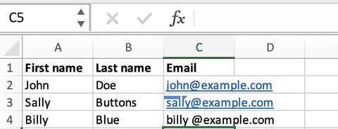
Sheet 2 has first name, last name, and phone number.

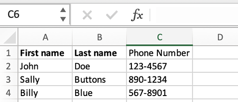
Let’s combine the data from the two sheets to make the data easier to work with.

First, let’s combine first and last names in case we have more than one John in our dataset.

1. Insert a new column in Sheets 1 and 2 to the right of the “last name” column.

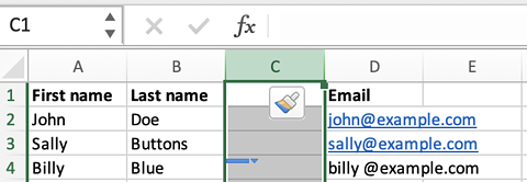
2. In C2 on both sheets, enter the formula:

=CONCATENATE(A2," ",B2)

(This says, for the string in A2, leave a space (” “) and then add the contents of B2.)

3. Select C2, click the bottom right corner of C2, and drag it to the bottom of your data to copy the formula down.

4. Now, insert a new column to the right of the combined name (C) in Sheet 1.

5. In the first row of the new column, enter the following formula:

=VLOOKUP(Sheet1!C2,Sheet2!$C:$E,2,FALSE)

This formula will search for whatever is in C2 in Sheet 2 (the full name of John Doe) and return the corresponding phone number to Sheet 1.

6. Copy the formula in the first row of the new column in Sheet 1 and paste it into the remaining rows in the column as you did with the concatenate formula.

Other Quick And Helpful Data Cleaning Commands

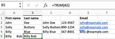
Want to remove unwanted space inside a cell? Use Trim. (It works in both Excel and Google Sheets.)

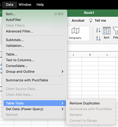
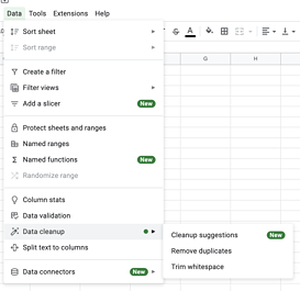
How To Combine Data Sets Into A Single Table Using Google Sheets

Another common task you’ll find yourself doing when working with data is getting all of it into the same sheet.

But a word of warning: Combining multiple data files can be a nightmare if you don’t prepare your data. So, make sure that they all have the same structure and format before you start.

Let’s start with something easy and work our way up.

Import One Entire Dataset Into Another

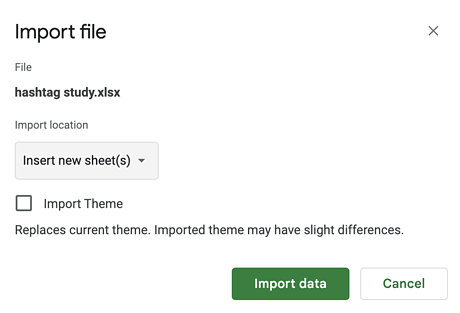
Import data into an existing sheet. File > Import> Select the data set to import > Insert. Then, change the dropdown to “Insert new sheet.” It will add the new data below.

Use The “QUERY” Function

Let’s say you have a sheet with traffic and bounce rates, and you want to create a sheet with bounce rates that are below 50% to identify your better-performing pages.

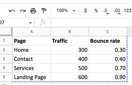
=QUERY(Sheet1!A2:C5, “SELECT A,B,C WHERE C < 0.5”)

This formula will create a new data set that includes all the information for any pages meeting our requirement of a 50% bounce rate.

In this formula, Sheet1!A2:C5 are the ranges it looks through; SELECT A,B,C tells it which cells to pull if the bounce rate is less than 0.5; and C < 0.5” is the math function that tells it to only copy the information from the other sheet if the value in column C is less than 0.5.

Use The “VLOOKUP” Function

The VLOOKUP function allows you to search for a value in one data set and return a corresponding value from another data set. Here’s an example of how to use it:

Two sheets: one with bounce rates (Sheet 2) and one with traffic numbers (Sheet 1).

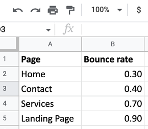
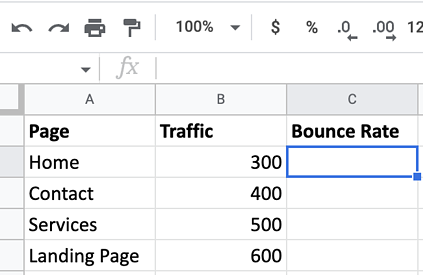
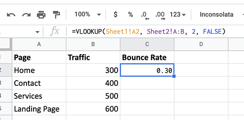
=VLOOKUP(Sheet1!A2, Sheet2!A:B, 2, FALSE)

This formula will search for the value in Sheet1!A2 in the first column of Sheet 2 and return the corresponding value from the second column of Sheet 2 when they match.

Your page names need to be the same on both sheets. If you have a “sale page” in one data set and a “landing page” on the other, it won’t work.

The “INDEX” And “MATCH” Functions

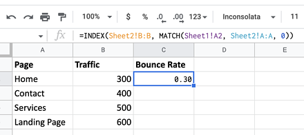
=INDEX(Sheet2!B:B, MATCH(Sheet1!A2, Sheet2!A:A, 0))

This formula will search for the value in Sheet1!A2 in the first column of Sheet 2 and return the corresponding value from the second column of Sheet 2.

Import Functions In The Formula Bar

IMPORTRANGE can get the job done from the formula bar.

=IMPORTRANGE(“spreadsheet_url”, “range_string”)

Copy the URL for the other data set. (Everything before the # sign.)

Then, tell it what range to copy across. (It will automatically update as changes are made on the other sheet.)

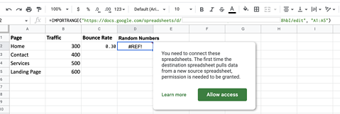
It will give you an error, so you just have to give it access. Other import types you can play with?

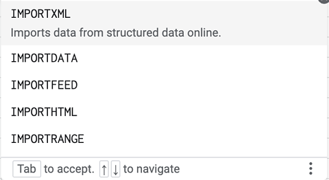
Import via RSS feed:

=IMPORTFEED(https://example.com/rss, “items title”)

Import via XML:

=IMPORTXML(“https://example.com/”, “xpath_query”)

Import via online structured data file (like a CSV):

=IMPORTDATA(“https://example.com/file.csv”)

Import from a table on a webpage:

=IMPORTHTML(“https://example.com/slug”,”table”,1)

(Where “table” is the query and “1” is the index start location.)

No-Formula Solutions

Google Sheets Add-Ons can also be really helpful if you’d like to avoid formulas. I’d encourage you to give the formulas a try, though. They’re flexible. (And they make you feel kind of smart and powerful when they work.)

How To Combine Data Sets Into A Single Table Using Excel

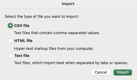
Simple Import

Choose File > Import > Select the data set. Then, tell it if it’s deliminated or a fixed width file. > Tell it how the file is delineated (tabs, colons, etc.). > Select data format (text, dates, etc.). > Finish.

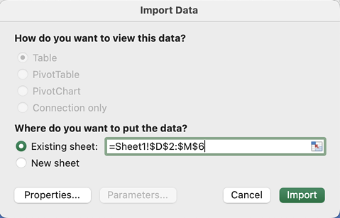
Finally, tell it if you want to add it to an existing sheet (and where), or if it should create a new sheet.

Use Excel’s Power Query

If you loved the query fetching in Google Sheets, you will love Power Query in Excel. Outside of Python, R, and learning an entire coding language, it is the most useful and powerful feature you can use to work with large data sets.

You’ll also find excellent documentation and plenty of videos (with data you can download to follow along with) to help you learn to use it. Monthly reporting data is an excellent practice.

Starting with a fresh Excel file? Import your data files straight into it.

Data > Get & Transform Data > Get Data. Select the file type to import or add via a URL and follow the prompts to import the file into Excel.

Continue to import all the data files into Excel.

Now, you need to combine the data files.

Data > Get & Transform Data > Combine Queries > Append Queries.

Select the ones you want. You can also add a custom column that identifies which file the data came from.

The VLOOKUP In Excel

The “VLOOKUP” function works just like VLOOKUP in Google Sheets. Here’s an example:

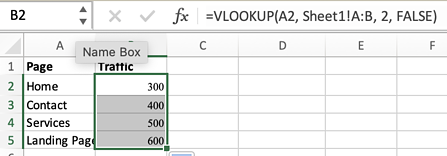
=VLOOKUP(A2, Sheet1!A:B, 2, FALSE)

This formula will search for the value in A2 in the first column of Sheet 2 and return the corresponding value from the second column of Sheet 2.

Use “INDEX” And “MATCH”

INDEX and MATCH work magic in Excel, too.

=INDEX(Sheet2!B5:C8,MATCH(Sheet1!A2,Sheet2!A5:A8,0)MATCH(D1,Sheet2!A4:C4,0))

This formula works by searching the range on Sheet 2 (in blue) by checking the first column (A5:A8) for whatever value is in A2 for an exact match (0). This is all the text in red.

The green text is the row information. It checks the first row (A4:C4) for whatever value it finds in D1, looking for an exact match (0).

Only want the value copied if the value is a certain amount? 1 = less than and -1 = more than.

If that doesn’t seem all that exciting, just wait until you see what you can do with this next.

Working With Data

Looking Up Values Using Two Customized Variables

Sometimes, you just want to be able to look up a specific value.

In this example, we have monthly traffic numbers in the columns and pages in the rows. Now, we can use INDEX and MATCH to look up how much traffic the contact page (or any page) received in the month of January (or any month) just by typing in G2 and G3.

The formula you put in G4:

=INDEX(B2:C5,MATCH(G3,A2:A5,0),MATCH(G2,B1:C1,0))

INDEX needs to know what range it should look in. Then, it wants to know which column and row it needs to find. The MATCH functions act as the row and column numbers by looking for exact matches according to what you typed in G2 and G3.

That means you can move that little typing section to a clean sheet and set up a dashboard so anyone on your team can look up data!

If you loved this, try it with SUMIFs and AVERAGEIFs, which sum (or average) data based on multiple criteria.

This is perfect for quickly summarizing your Google Analytics data based on specific criteria, such as traffic source, medium, and date range.

Create Pivot Tables

Pivot tables are likely one of the most important tools you’ll have when trying to summarize large amounts of data and transform it into a more manageable format.

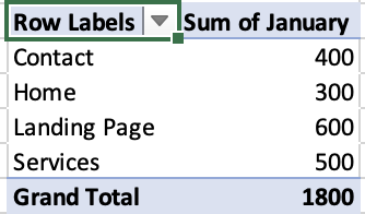
Use it to speed up your reporting by:

• Summarize traffic data by product, category, or time period.
• Analyze traffic over time to identify seasonal trends.
• Compare data across different categories, such as bounce rates for the landing pages for different products or regions.
• Filter data to show only data for a specific product or region.
• Calculate metrics such as averages, counts, and percentages. For example, the average traffic per day for each product over the last 30 days.
• Identify outliers such as pages or products that are selling much more or much less than other products.

In Google Sheets:

Highlight the data you want to analyze.

To make the table: Data > Pivot Table to open a new sheet with a blank pivot table.

Now, set up your pivot table.

In the “Rows” and “Columns” fields, select the fields you want to use as rows and columns. In the “Values” field, select the field you want to analyze.

Need something a little different? Customize your pivot table by changing the summary function (sum, average, count, for example), sort and filter the data, and add subtotals and grand totals.

Pro Tip: Have a large data set? Select the entire table by clicking on the top-left corner of the table.

In Excel:

Same as in sheets, start by highlighting the data you want to analyze. For a large data set, clicking on the top-left corner of the table works here, too.

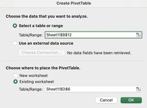
Insert > Pivot Table > Insert the range where your data is that you want to analyze. Then, if you want the pivot table on a new sheet or in the existing one.

(If you accidentally selected an empty range, it will give you an error. So, if it complains, this is usually why.)

Now, set up your pivot table. Add whatever you want in the columns into the “Values” field and the rows into the “Rows” field.

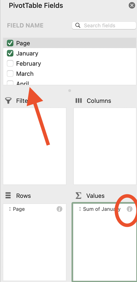
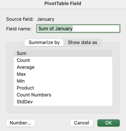
And if you need to change it (so it’s using average instead of sum, for example), change that using the information button on the appropriate value.

Use REGEXTRACT To Pull Information From URLs

The Regexextract formula extracts specific data from text strings using regular expressions. So, for example, you can use Regexextract to extract the source and medium of your website traffic from Google Analytics reports.

To extract the domain from a URL in cell A2, you can use the following formula:

=REGEXEXTRACT(A2,”^(?:https?://)?(?:[^@\n]+@)?(?:www.)?([^:/\n]+)”)

Regular expressions can be complex, so it’s important to test your formula with different examples to ensure it is extracting the correct data.

Minimizing Tables

To minimize a table, click on the small arrow icon in the top left corner of the table to collapse it and hide the data, leaving only the table header visible.

To expand the table again, simply click on the arrow icon.

You can also use the “Data” > “Group Rows” or “Group Columns” feature to group related rows or columns together and create collapsible sections.

Freezing Rows And Columns

Freezing rows and columns keeps specific rows or columns visible on the screen while you scroll through the rest of the spreadsheet.

In Google Sheets: Select the row or column you want to freeze. Click View > Freeze > Up to current row or column (or up to and including the current row/column.)

In Excel: Select the row or column you want to freeze. Then, click View > “Freeze Panes,” “Freeze Top Row,” or “Freeze First Column.”

If you’re really struggling with a large amount of data, try filters. This allows you to remove any irrelevant data and show only the data that meets certain criteria.

Extra Tips For Large Data Sets

Use named ranges to assign a specific name to a range of cells in your sheet. This can make it easier to refer to and analyze large data sets.

Avoid using too many formulas. These slow down your sheet’s performance and can also make your life very difficult, particularly once you start chaining multiple formulas together.

Make use of conditional formatting:

In Google Sheets:

Select the range of cells you want to apply conditional formatting to. Click Format > Conditional Formatting.

In the “Conditional format rules” panel on the right-hand side of the screen, select the type of formatting you want to apply. There are several options to choose from, including “Color scale,” “Icon set,” and “Custom formula is.”

In Excel:

Select the range of cells you want to apply conditional formatting to and click Home > Styles > Conditional Formatting.

In the drop-down menu, select the type of formatting you want to apply, including “Highlight Cells Rules,” “Top/Bottom Rules,” and “Data Bars.”

Conclusion

Excel and Google Sheets may look too simplistic to do much, or they might appear too complicated to learn, but neither of those assumptions is true.

With a few formulas and tricks up your sleeve, you’ll quickly find they’re among the most powerful and important tools in your SEO toolbox.

Ready to become a data pro? Download The Complete Technical SEO Audit Workbook and master the art of preparing and working with data.

Featured Image: Paulo Bobita/Search Engine Journal

In-post Images: Screenshot by author from Excel/Google Sheets, May 2023